Monte Carlo Simulation for your portfolio: a practical guide
How Monte Carlo simulation works applied to investment portfolios: scenarios, fan charts, withdrawals and probability of success explained step by step.
Sunday, 15 March 2026

The problem with average returns
Suppose you have a portfolio of €100,000 with an expected average return of 7% per year. After 20 years, linear projection says:
$$V_{20} = 100,000 \times (1.07)^{20} \approx 386,968 \text{ €}$$
The number looks precise. But it hides a lie: markets don’t grow 7% every year in an orderly fashion. One year they’re up 22%, the next down 18%, then up 11%. The sequence matters, and the average doesn’t capture it.
Monte Carlo simulation serves exactly this purpose: to replace linear projection with thousands of plausible scenarios, each with its own sequence of random returns.
What is Monte Carlo simulation
Monte Carlo simulation is a statistical technique that generates a large number of future scenarios by randomly sampling from a probability distribution.
In finance it is used to answer questions like:
- What is the probability that my portfolio reaches €300,000 in 20 years?
- With what probability can I withdraw €500 a month for 30 years without running out of capital?
- What percentile of outcome should I expect in the pessimistic scenario?
The name comes from the Monte Carlo casino: just as repeated dice rolls generate a distribution of outcomes, simulation repeats the “roll” of market returns thousands of times.
How it works: the steps
1. Define the model parameters
For each asset or portfolio, three fundamental inputs are needed:
- Expected annual return ($\mu$): estimate based on historical data or forward expectations.
- Annual volatility ($\sigma$): standard deviation of returns.
- Time horizon ($T$): number of years for the simulation.
2. Generate random returns
The simplest model assumes that annual returns follow a normal distribution:
$$r_t \sim \mathcal{N}(\mu,, \sigma^2)$$
For each simulation $i$ and each year $t$, a random return $r_{i,t}$ is drawn.
3. Calculate the portfolio path
The portfolio value at the end of each year is updated by multiplying by the realized return:
$$V_{i,t} = V_{i,t-1} \times (1 + r_{i,t})$$
Repeating for $N$ simulations (typically 1,000 to 10,000) yields a distribution of possible paths.
4. Read results by percentiles
Rather than a single number, the result is a distribution:
| Percentile | Meaning |
|---|---|
| 10th | Only 10% of scenarios perform worse than this |
| 25th | Unfavorable scenario but not extreme |
| 50th | Median scenario (half of scenarios above, half below) |
| 75th | Favorable scenario |
| 90th | Only 10% of scenarios perform better than this |
Practical example: €100,000 for 20 years
Parameters: initial capital €100,000, expected return 7%, volatility 14%, horizon 20 years, 1,000 simulations.
Fan chart: all possible paths
The following chart shows the 1,000 simulated paths overlaid. The colored bands represent key percentiles.
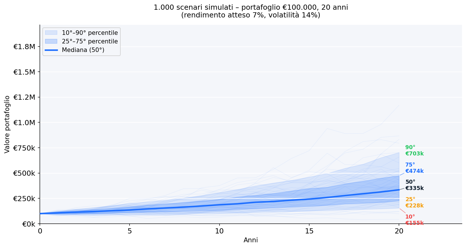
What to observe:
- The central band (25th–75th percentile) covers the majority of realistic scenarios.
- Dispersion grows over time: uncertainty accumulates.
- Even in the 10th percentile scenario, capital does not go to zero, because no withdrawals are made.
Distribution of final values
After 20 years, the distribution of final values from the 1,000 simulations looks like this:

The three key values to read:
- 10th percentile: pessimistic scenario on which to size risk
- 50th percentile (median): realistic central expectation
- 90th percentile: optimistic scenario not to be taken for granted
The distribution is not symmetric: the right tail (extreme gains) is longer than the left tail (extreme losses), because the portfolio cannot fall below zero but can grow indefinitely.
Monte Carlo for withdrawal planning
The most powerful application of Monte Carlo simulation concerns the decumulation phase: how much money can you withdraw each year without risking running out of portfolio?
The classic question: a capital of €100,000 over a 30-year horizon, with a fixed annual withdrawal, what is the probability of success (portfolio > 0 at the end)?
The chart below compares different withdrawal rates:
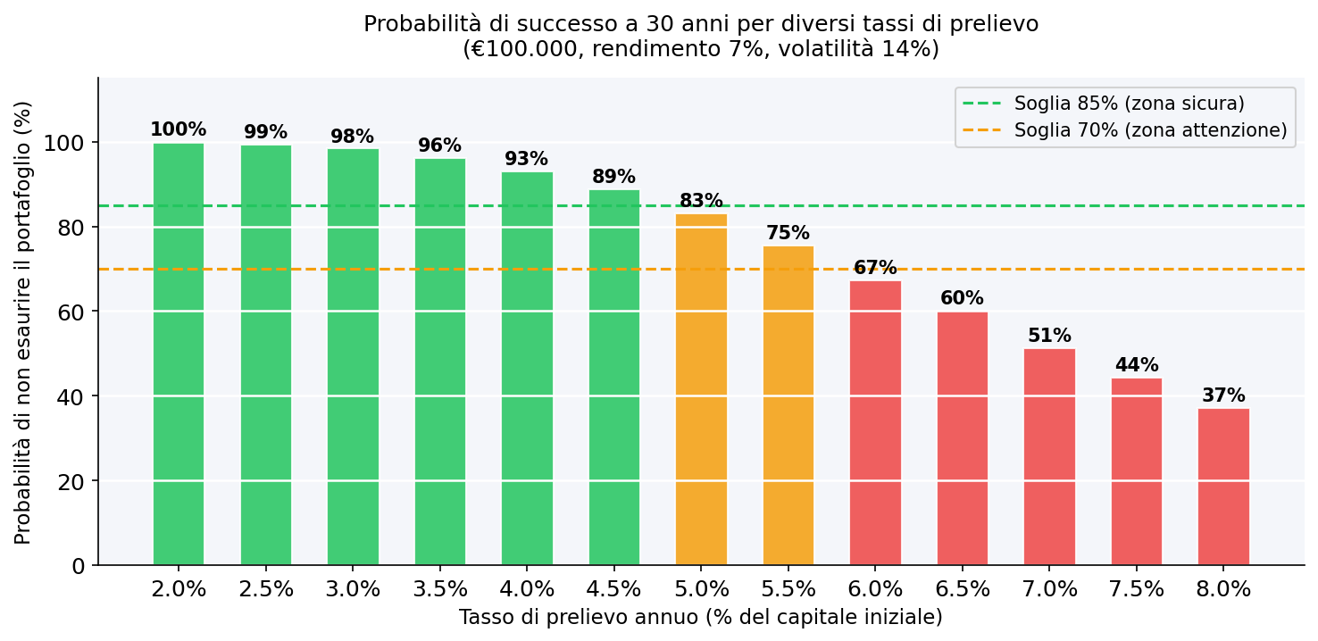
The practical reading:
- Up to 3.5% per year: very high probability of success (green zone). With €100,000 that means no more than €3,500/year.
- Between 4% and 5%: caution zone. The outcome depends heavily on the actual sequence of returns in the early years.
- Over 5.5%: the probability of depleting the portfolio before 30 years becomes significant.
This is the quantitative foundation of the so-called 4% rule (elaborated by Bengen’s studies in 1994 on U.S. markets): with annual withdrawals equal to 4% of initial capital, the historical probability of success over 30 years was very high. Parameters vary for European markets and portfolios with different volatilities.
Variant: Monte Carlo with monthly withdrawals and inflation
A more realistic model includes two adjustments:
Withdrawal adjusted for inflation: each year the withdrawal increases in line with expected inflation $\pi$:
$$W_t = W_0 \times (1 + \pi)^t$$
Portfolio with monthly withdrawal: the value is updated each month by subtracting the monthly withdrawal $W_t / 12$:
$$V_{i,t} = V_{i,t-1} \times (1 + r_{i,t}) - \frac{W_t}{12}$$
These two adjustments lower the probability of success compared to the base model, making the estimate more conservative and reliable.
Limitations of Monte Carlo simulation
Monte Carlo simulation is a powerful tool, but it should be used with awareness of its limitations.
Dependence on input parameters: if you overestimate expected return or underestimate volatility, results will be optimistic. Garbage in, garbage out.
Normal distribution vs. reality: real markets show thicker tails than normal (high kurtosis) and negative skewness. A model based only on mean and standard deviation can underestimate extreme negative events.
Absence of dynamic correlations: in a crisis, correlations between assets tend to increase. A model that uses stable historical correlations may underestimate risk in stress scenarios.
The sequence matters more than the average: two portfolios with the same average annual return can have very different results if the sequence of negative years changes. This is particularly critical in the withdrawal phase (sequence of returns risk).
To overcome these limitations, more sophisticated variants are used: simulations based on real historical returns (bootstrap), GARCH models for time-varying volatility, or multi-asset models with dynamic covariance matrices.
How to read Monte Carlo simulation in practice
When you use a tool that shows you Monte Carlo output, keep these principles in mind.
Don’t fixate on the median value as if it were a certainty: the 50th percentile means that half of the scenarios perform worse. For personal financial planning, consider the 25th or 10th percentile as a reference for conservative decisions.
Use percentiles to answer precise questions: “what is my probability of reaching X?” is more useful than “what is the expected value?”.
Update the simulation periodically: as your portfolio grows or changes, or as market conditions change, input parameters should be recalibrated.
Integrate with other risk metrics: Monte Carlo simulation works well alongside VaR and CVaR, maximum drawdown, and skewness/kurtosis.
Frequently asked questions
Is Monte Carlo simulation reliable for deciding how much to withdraw in retirement?
It is the most robust tool available for this purpose, but it is not infallible. Results depend on the parameters used and the return distribution model. Use it as a quantitative compass, not as a guarantee. Always add a margin of safety relative to the probability of success you deem acceptable.
How many simulations do I need for stable results?
Generally, 1,000 simulations already give stable results for planning purposes. With 10,000, convergence is practically complete. Adding simulations beyond this threshold does not significantly change percentiles.
What is the difference between historical Monte Carlo and parametric Monte Carlo?
Parametric Monte Carlo draws returns from a theoretical distribution (e.g., normal) with estimated mean and standard deviation. Historical Monte Carlo samples actual past returns directly (bootstrap), preserving actual tails, skewness, and correlations. The second is generally more conservative and realistic.
Can I use Monte Carlo simulation for multi-asset portfolios?
Yes, but you need a covariance matrix to capture correlations between assets. A stock/bond portfolio behaves differently than an all-stock one because the two components don’t move in perfect synchronization.
What does “90% success probability” mean in a withdrawal plan?
It means that in 9 out of 10 simulations, the portfolio does not run out before the end of the time horizon. It is not an absolute guarantee, but in 1 out of 10 scenarios the portfolio could run out before. The acceptable threshold depends on risk tolerance and the presence of other income sources (public pension, real estate, etc.).
Does the 4% rule work in Italy or Europe?
The 4% rule was developed on historical U.S. data (S&P 500 + U.S. bonds). For European markets, with slightly lower historical returns and different valuations, many analysts suggest using a more conservative withdrawal rate, around 3%–3.5%, in the absence of other income sources.
Next steps
- Analyze your portfolio risk in the Wallible app
- Compare scenarios with the ETF portfolio simulator
- Explore tail risk with VaR and CVaR and Expected Shortfall
- Read about return distribution with skewness and kurtosis
- Understand maximum drawdown as a complement to simulation
Related guides
TWR vs MWRR: which return metric should you trust?
TWR and MWRR measure portfolio returns differently. Learn which metric applies to your situation and why using the wrong …
Skewness and Kurtosis: practical guide for portfolio risk
Understand skewness and kurtosis, how to read return-distribution shape, and why tails matter for risk decisions.
Expected Shortfall (CVaR) 95% and 99%: practical guide
Understand CVaR 95% and 99%, how it differs from VaR, and how to use tail-risk metrics for portfolio decisions.